Data visualisation

Artificial Intelligence, Data Governance, Data Marketing, Data Mining and Data Integration, Data visualisation

DATA: 7 Pitfalls to Avoid, Ep 7/7 – Design dangers

The Critical Role of Design in Data Presentation

As Steve Jobs once said, « Design is not just what it looks like and feels like. Design is how it works. » This principle applies perfectly to data visualization. In this final episode of our series, we’ll explore the often-overlooked dangers related to design in data presentation.

Pitfall 7A: Confusing colors

Color choice is a crucial aspect of data visualization design, yet it’s often mishandled. Poorly chosen colors can make visualizations difficult to read or even misleading. Here are some common color-related pitfalls:

  1. Using too many colors: This can visually overwhelm and make understanding difficult.
  2. Choosing colors that don’t contrast well: This can make it challenging to differentiate between categories.
  3. Ignoring color blindness: Some color combinations can be indistinguishable for color-blind individuals.
  4. Using the same color for different variables: This can lead to confusion and misinterpretation.

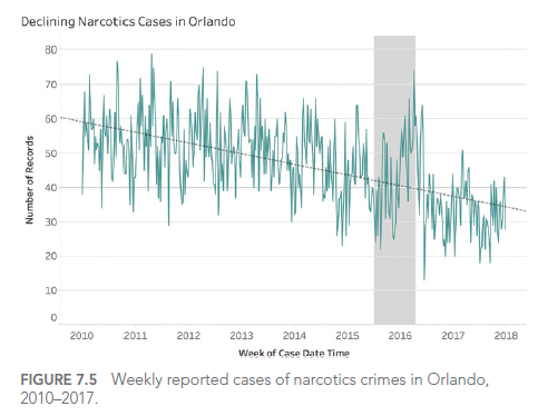
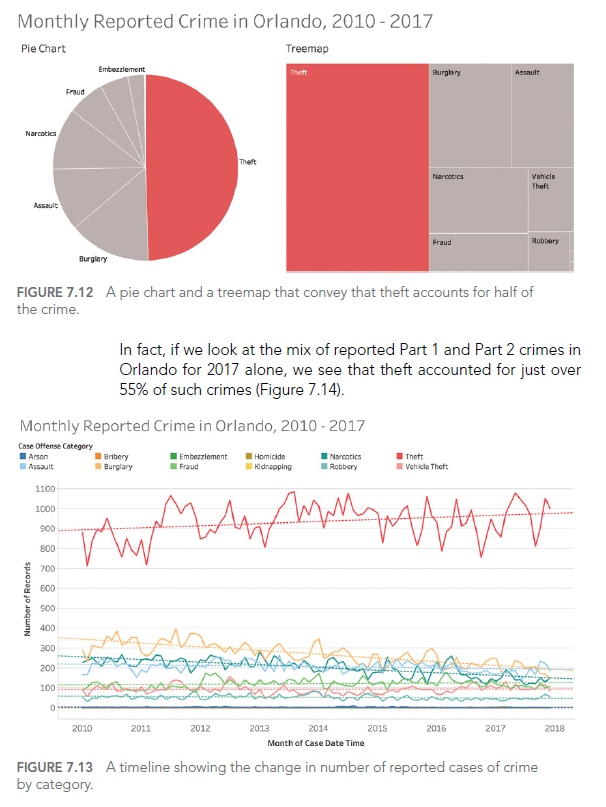
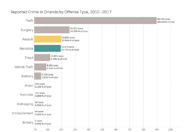
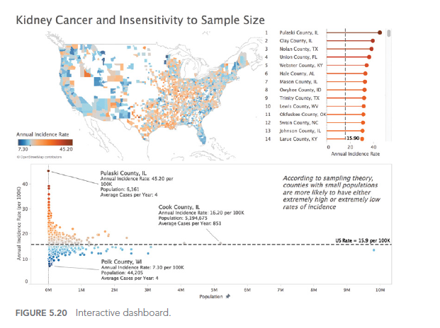
Consider this example of a poorly designed dashboard:

In this dashboard, the use of similar colors for different categories makes it difficult to distinguish between crime types. A better approach would be to use a clear, distinct color palette with high contrast between categories.

Pitfall 7B: Missed opportunities

Sometimes, in our quest for simplicity, we miss opportunities to enhance understanding through design. Thoughtful addition of visual elements can greatly improve engagement and memorability.

For example, consider this improved visualization of Edgar Allan Poe’s works:

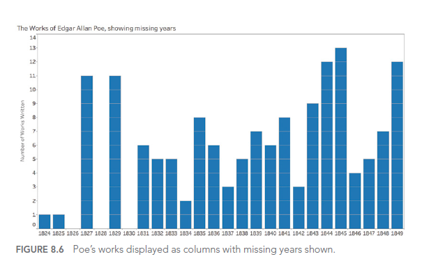
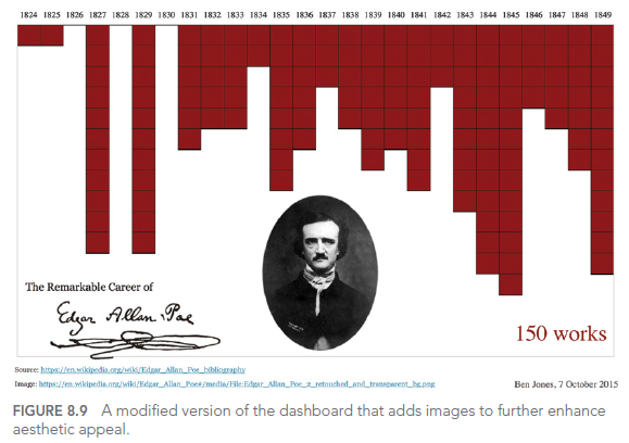
This visualization uses design elements to evoke the dark ambiance of Poe’s works, making the visualization more memorable and engaging. The inverted y-axis and blood-red color scheme add to the ominous feel, while the portrait and signature provide context and personality.

Pitfall 7C: Usability Uh-Ohs

Good design isn’t just about visual appeal; it must also consider usability. Visualizations that are difficult to manipulate or understand can frustrate users and limit the effectiveness of data communication.

Key usability considerations include:

  • Intuitive navigation: Users should easily understand how to interact with the visualization.
  • Clear labeling: All elements should be clearly labeled to avoid confusion.
  • Responsive design: Visualizations should work well on various devices and screen sizes.
  • Accessibility: Design should accommodate users with different abilities.

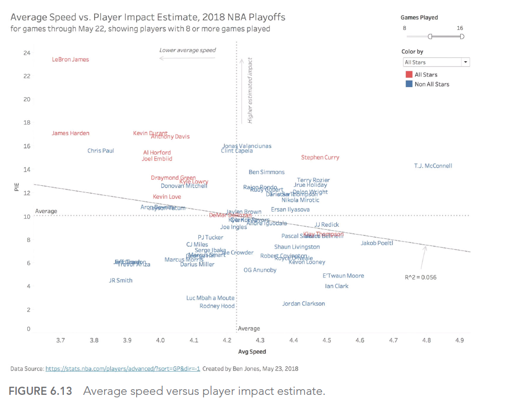
Here’s an example of a dashboard with potential usability issues:

While this dashboard offers numerous interaction options, without careful user interface design, it can become overwhelming and difficult to use effectively. A better approach would be to simplify the interface, prioritize key information, and provide clear guidance on how to interact with the visualization.

CONCLUSION

In this final article of our series, we’ve explored the seventh type of error we can encounter when working with data: design dangers. We’ve seen how color choices, missed opportunities, and usability issues can affect the effectiveness of our data visualizations.

Throughout this seven-part series, we’ve covered a wide range of common pitfalls in working with data, from how we think about data to how we present it. By being aware of these pitfalls and learning how to avoid them, we can significantly improve our ability to work effectively with data and communicate valuable insights.

Remember, good design in data visualization is not just about making things look pretty. It’s about enhancing understanding, facilitating insights, and enabling better decision-making. As you continue your data journey, keep these principles in mind to create visualizations that are not only visually appealing but also clear, informative, and user-friendly.

This series of articles is strongly inspired by the book « Avoiding Data Pitfalls – How to Steer Clear of Common Blunders When Working with Data and Presenting Analysis and Visualizations » written by Ben Jones, Founder and CEO of Data Literacy, WILEY edition. We highly recommend this excellent read to deepen your understanding of data-related pitfalls and how to avoid them!

You can find all the topics covered in this series here: https://www.businesslab.mu/blog/artificial-intelligence/data-7-pitfalls-to-avoid-the-introduction/

Data Governance, Data Marketing, Data Mining and Data Integration, Data visualisation, Machine Learning, Self-service Analytics

DATA: 7 Pitfalls to Avoid, Ep 6/7 – Graphical blunders

How to Avoid Common Errors in Data Visualization

Data visualization is a powerful tool for communicating complex information clearly and concisely. However, it can also be a source of numerous errors that can lead to misinterpretations. In this episode, we’ll explore the most common graphical gaffes and how to avoid them.

Pitfall 6A: Misleading Graphs

One of the most common pitfalls in data visualization is creating graphs that mislead, often unintentionally. This can happen in several ways:

  1. Truncating the Y-axis: By not starting the Y-axis at zero, visual differences between values can be exaggerated.
  2. Choosing an inappropriate scale: A poorly chosen scale can hide or exaggerate important trends.
  3. Using 3D graphs: 3D graphs can distort the perception of proportions.

For example, consider this graph showing drug-related crime cases in Orlando:

This graph seems to show an alarming increase in drug-related crimes. However, upon closer examination, we see that the Y-axis doesn’t start at zero, visually exaggerating the increase.

Pitfall 6B: Data Dogmatism

It’s easy to fall into the trap of data dogmatism, thinking there’s only one « right » way to visualize data. In reality, the choice of graph type depends on the context, audience, and message you want to convey.

For example, although pie charts are often criticized, they can be effective for showing parts of a whole, especially when there are few categories:

This pie chart clearly shows that theft accounts for nearly half of all reported crimes in Orlando.

Pitfall 6C: The false optimization/satisfaction dichotomy

In data visualization, one can fall into the trap of thinking that we must always seek the « optimal » visualization at the expense of « satisfactory » solutions. In reality, it’s often more practical and effective to find a visualization that meets the needs sufficiently well, rather than spending excessive time seeking perfection.

For example, this horizontal bar chart can be « satisfactory » for showing the most common types of crimes, even if it’s not necessarily « optimal »:

This graph is easy to understand and quickly provides essential information, even if it could potentially be optimized further.

CONCLUSION

In this article, we explored the sixth type of error we can encounter when working with data: graphical gaffes. We’ve seen how to avoid misleading graphs, data dogmatism, and the false dichotomy between optimization and satisfaction.

In the next and final article in our series, we’ll explore the 7th type of error: design dangers. We’ll see how design choices can affect the perception and interpretation of visualized data.

This series of articles is strongly inspired by the book « Avoiding Data Pitfalls – How to Steer Clear of Common Blunders When Working with Data and Presenting Analysis and Visualizations » written by Ben Jones, Founder and CEO of Data Literacy, WILEY edition. We highly recommend this excellent read to deepen your understanding of data-related pitfalls and how to avoid them!

You can find all the topics covered in this series here: https://www.businesslab.mu/blog/artificial-intelligence/data-7-pitfalls-to-avoid-the-introduction/

Business Intelligence, Data Governance, Data Marketing, Data Mining and Data Integration, Data Quality Management, Data Regulations, Data visualisation, Machine Learning, Self-service Analytics

DATA: 7 Pitfalls to Avoid, Ep 5/7 – Analytical aberrations

Intuition and Analysis are Not Mutually Exclusive

In our quest to make the most of data, we often fall into the trap of considering intuition and analysis as mutually exclusive approaches. However, as we’ll see in this episode on analytical aberrations, intuition plays a crucial role in the data analysis process.

Pitfall 5A: the False Intuition/Analysis Dichotomy

There was a time when advertisements boasted about moving from intuition to analysis in decision-making. This view is mistaken. Intuition isn’t obsolete in the data age – it’s actually more valuable than ever.

Intuition is the spark that powers the engine of analysis. It helps us:

  1. Know WHY the data is important
  2. Understand WHAT the data is telling us (and isn’t telling us)
  3. Know WHERE to look next
  4. Know WHEN to stop analyzing and take action
  5. Know WHO needs to hear the results and HOW to communicate them

Pitfall 5B: Exuberant Extrapolations

Predicting the future from data can be risky. Extrapolating current trends can lead to significant errors if we don’t account for natural limits or potential changes.

For example, if we look at life expectancy in North and South Korea from 1960 to 1980, we might be tempted to predict a continuous, linear increase. However, reality turned out quite differently, especially for North Korea, which experienced a significant decline in the 1990s.

Pitfall 5C: Ill-Advised Interpolations

When working with time-series data, we must be careful in our interpretations between data points. A simple slope graph connecting two points in time can mask significant fluctuations between these points.

For example, consider life expectancy in certain countries between 1960 and 2015. A simple slope graph showing the change between these two years could give the impression of a steady and constant increase. However, this simplified representation would mask periods of conflict, economic hardship, or rapid progress in public health that significantly impacted life expectancy over the years.

Take the case of Cambodia, Timor-Leste, Sierra Leone, and Rwanda. A simple slope graph would show an increase in life expectancy between 1960 and 2015, but would completely obscure the tragic periods of war and genocide these countries experienced. For instance, life expectancy in Cambodia fell to less than 20 years in 1977 and 1978, a crucial fact that would be completely ignored in a simple interpolation between 1960 and 2015.

This graph shows the actual evolution of life expectancy in these countries, revealing the dramatic fluctuations masked by a simple linear interpolation.

Pitfall 5D: Funky Forecasts

Forecasts, especially long-term ones, can be particularly prone to errors. A striking example is the unemployment forecasts made by different U.S. presidential administrations. These forecasts tend to show a rapid return to a « normal » rate of 4-6%, regardless of the actual economic situation.

This phenomenon can be explained by several factors. First, there’s political pressure to present optimistic outlooks. Second, there’s a natural tendency to assume that extreme or unusual situations will correct themselves quickly. Finally, forecasting models are often based on historical data and may not adequately account for structural changes in the economy.

For example, during the 2008 financial crisis, unemployment forecasts made just before or at the beginning of the crisis failed to anticipate the magnitude and duration of the increase in unemployment. Similarly, forecasts made at the height of the crisis often underestimated the time it would take for the unemployment rate to return to pre-crisis levels.

This graph shows how different presidential administrations have consistently predicted a rapid return to a « normal » unemployment rate, even in the face of very different economic realities.

Pitfall 5E: Moronic Measures

It’s crucial to ensure that the measures we use are relevant and meaningful. Too often, we focus on measures that are easy to obtain rather than those that are truly important for understanding a phenomenon or making decisions.

In sports, for example, many traditional measures can be misleading. Take the case of professional basketball: a player’s average speed on the court might seem like an interesting measure, but it doesn’t necessarily reflect the player’s real impact on the game.

LeBron James, one of the best players of all time, was criticized during the 2018 playoffs for having the lowest average speed on the court. However, this measure didn’t account for his real impact on the game, measured by more relevant statistics like the Player Impact Estimate (PIE).

This graph shows the relationship between average speed and PIE for NBA players. We can see that LeBron James (point in the top left) has a very high PIE despite a relatively low average speed, illustrating why average speed alone is an inadequate measure of a player’s performance.

This case illustrates the importance of choosing measures that truly reflect what we’re trying to evaluate, rather than settling for measures that are easy to obtain but potentially misleading.

In this article, we explored the fifth type of error we can encounter when using data to illuminate the world around us: analytical aberrations. We’ve seen how intuition and analysis can work together, and how to avoid the pitfalls of exuberant extrapolations, ill-advised interpolations, funky forecasts, and moronic measures.

In the next article, we’ll explore the 6th type of error in our series: graphical gaffes. We’ll see how errors in data visualization can lead to misinterpretations and poorly informed decisions.

This series of articles is strongly inspired by the book « Avoiding Data Pitfalls – How to Steer Clear of Common Blunders When Working with Data and Presenting Analysis and Visualizations » written by Ben Jones, Founder and CEO of Data Literacy, WILEY edition. We highly recommend this excellent read to deepen your understanding of data-related pitfalls and how to avoid them!

You can find all the topics covered in this series here: https://www.businesslab.mu/blog/artificial-intelligence/data-7-pitfalls-to-avoid-the-introduction/

Artificial Intelligence, Business Intelligence, Data Governance, Data Marketing, Data Mining and Data Integration, Data Quality Management, Data Regulations, Data visualisation, Machine Learning, Self-service Analytics

DATA: 7 pitfalls to avoid, Ep 4/7 – Statistical errors – Facts are stubborn things, but statistics are malleable

“There are lies, damned lies and statistics” B.Disraeli


Why such distaste for a field that, according to Webster’s Merriam-dictionary, is simply “a branch of mathematics dealing with the collection, analysis, interpretation and presentation of masses of numerical data. ”1 Why is the field of statistics in such a negative light by so many people?

There are four main reasons

  • It’s a complex field. Even the basic concepts are not easily accessible and are very difficult to explain.
  • Even the best-intentioned experts can misapply the tools at their disposal.
  • The third reason behind all this hatred is that those with an agenda can easily create statistics to lie about when communicating with us.
  • The final reason is that statistics can often seem cold and distant, making them very difficult for the public to grasp.

Descriptive setbacks

Descriptive statistics are intended to summarize the main characteristics of a data set. However, incorrect or inappropriate use can lead to misleading conclusions. A typical example is the use of the mean to summarize a distribution, without taking into account variability or skewness. Another common error is to present percentages without explaining the total number of people, which can be misleading as to the true extent of a phenomenon. It is therefore crucial to understand the assumptions and limitations of each descriptive measure in order to use it correctly.

Let’s take the example of analyzing salaries within a company. If we simply look at average salaries, we might conclude that the company is paying its employees well. However, if management salaries are very high compared to the rest of the employees, the average would be biased upwards. It would be more relevant to use the median, which gives the salary in the middle, or to look at the complete salary distribution for a more accurate view.

This error is very well described here with cats:

Inferential fires

Always a feline explanation:

Statistical inference aims to draw conclusions about a population from a sample of that population. However, this process is subject to error. Sampling errors and Type I and II errors are common. In addition, errors can be exacerbated by confusion between correlation and causation. A solid understanding of the principles of statistical inference is essential to avoid these pitfalls.

Let’s imagine a public health study seeking to establish a link between a particular dietary habit (such as eating organic) and better overall health. If the study finds a positive correlation, it doesn’t necessarily mean that eating organic causes better health. There could be confounding factors, such as income level or lifestyle, that influence both eating habits and health status. Here, we can fall into the trap of confusing correlation with causation.

Sliding sampling

Sampling is a crucial stage in any data collection process. Yet many errors can occur at this stage. The sample may not be representative of the target population, due to selection bias or non-response. What’s more, the sample size may be insufficient to detect an effect. Careful sample planning is therefore essential to obtain reliable results.

Consider a customer satisfaction survey conducted by an e-commerce company. If the company only solicits opinions from customers who have made a recent purchase, it runs the risk of obtaining a distorted picture of overall customer satisfaction. Indeed, dissatisfied customers may have stopped making purchases and therefore not be included in the sample. This is an example of selection bias.

Insensitivity to sample size

A common mistake in data analysis is to ignore the impact of sample size on results. A large sample size can make a very small effect significant, while too small a sample size may not have sufficient power to detect an existing effect. Furthermore, statistical significance does not necessarily mean practical significance. So it’s important to consider sample size when interpreting results.

Suppose you’re conducting a study to assess the effect of a drug on lowering blood pressure. If you have a very large sample of patients, you may see a statistically significant drop in blood pressure. However, this drop may be very small, say 0.1 mm Hg, a clinically insignificant value despite its statistical significance. This is an example where sample size can make a small effect significant. On the other hand, if the sample is too small, a real effect may be missed. It is therefore important to consider clinical or practical significance in addition to statistical significance.

Digging deeper into this issue, Ben Jones (see author who inspired this article) managed to find figures on kidney cancer rates as well as demographics for every US county, and he created an interactive dashboard (figure below) to visually illustrate the fact that Kahneman, Wainer and Zwerlink are doing quite clearly in words.

Notice a few elements in the dashboard. On the choropleth map (filled in), the darkest orange counties (high rates relative to the overall U.S. rate) and the darkest blue counties (low rates relative to the overall U.S. rate) are often side by side.

Also, note how in the scatterplot below the map, the marks form a funnel shape, with less populated counties (on the left) more likely to deviate from the reference line (the overall U.S. rate), and more populated counties like Chicago, L.A. and New York are more likely to be close to the overall reference line.


One final observation: if you hover over a county with a small population in the interactive online version, you’ll notice that the average number of cases per year is extremely low, sometimes 4 cases or less. A small deviation – even just 1 or 2 cases – in a subsequent year will pull a county from the bottom of the list to the top, or vice versa.


In the next article, we’ll explore the 5th type of error we may encounter when using data to illuminate the world around us: Analytical aberrations.

This article is heavily inspired by the book “Avoiding Data pitfalls – How to steer clear of common blunders when working with Data and presenting Analysis and visualization” written by Ben Jones, Founder and CEO of Data Litercy, WILEY edition. We recommend this excellent read!

You can find all the topics covered in this series here: https://www.businesslab.mu/blog/artificial-intelligence/data-7-pitfalls-to-avoid-the-introduction/